Mesh Quallity
Mesh quality

• For
the same cell count, hexahedral meshes will give more
Accurate solutions,
especially if the grid lines are aligned with the
Flow.
• The
mesh density should be high enough to capture all relevant
Flow features.
• The
mesh adjacent to the wall should be fine enough to resolve
The boundary layer
flow. In boundary layers, quad, hex, and
Prism/wedge cells are
preferred over tri’s, tets, or pyramids.
• Three
measures of quality:
– Skewness.
– Smoothness
(change in size).
– Aspect
ratio.
Skewness
Two methods to define skewness are:
·
Based on equilateral volume :
o
Skewness = (optimal cell size – actual
cell size) / (optimal cell size)


o
Applied to only tri and tet meshing.
o
This method on meshing follows Delaunay
triangulation theorem.
o
Default method used in ansys for tri and
tet meshing.
·
Based on the deviation from a normalized
equilateral angle
o
Skewness = Max [ {(θmax -90)/
90}, {(90 – θmin )/90}]


o
Applies to all cell and face shapes,
used generally for quads.
o
Used for prisms, pyramids, etc.
Smoothness
and aspect ratio
- Change is mesh size should be gradual or smooth

- Aspect ratio is the ratio of longest edge length to the shortest edge length. It is equal to 1 for an equilateral triangle or square.


Checking For Quality


·
Solver Study: Turbulent Flow Models
Turbulence or turbulent flow is a flow characterised by random and chaotic fluid flow with unexpected property changes.

Turbulence Models
A turbulence modelling is a computational procedure to close the system of mean flow equations. For most engineering applications it is unnecessary to resolve the details of turbulent fluctuations. Turbulence models allow the calculation of the mean flow without first calculating the full time-dependent flow field. we only need to know how turbulence affected the mean flow.
The classical turbulence models are based on the Reynolds Averaged Navier-Stokes equations (RANS) :
One equation model: Spalart-Allmaras
- Two equation model: -> k-epsilon (Standard, RNG and realizable)
-> k-omega - Seven equation: Reynolds stress model (RSM)

This model solves a single conservation equation (PDE) for the turbulent viscosity. It contains both connective and diffusive transport terms as well as expressions for the productive dissipation of turbulent viscosity.
It was developed for the use in unstructured codes in the aerospace industry. It gives accurate results for attached wall-bounded flows and flows with mild separation and recirculation. however it gives improper results for massively separated flows, free shear flows and decaying turbulence.
Can be used for:
- Drag prediction with mild turbulence
- Wing parameter calculation for mild separation conditions

The transport variable used in the equations is the turbulent kinetic energy. The second transported variable in this case is the turbulent dissipation (epsilon). The K-epsilon model has been shown to be useful for free-shear layer flows with relatively small pressure gradients. Similarly, for wall-bounded and internal flows, the model gives good results only in cases where mean pressure gradients are small; accuracy has been shown experimentally to be reduced for flows containing large adverse pressure gradients. It has 3 variations :
- Standard k epsilon model: Good for simple simulations
- Realisable k epsilon model : Improved performance for flows involving boundary layers under strong adverse pressure gradients or separation, rotation, re circulation and strong streamline curvature
- RNG k epsilon model : It offers improved accuracy in rotating flows, favoured for indoor air simulations. better results for rotating flow and effect of swirl on turbulence
although it is not favored for rotating and swirling flows.
k omega 2 equation model

It is another 2 equation model similar to k epsilon model which solves 2 additional PDE's resulting in a faster converging solution. however it is not widely used because it might give errors(An assumption based on trial and error)
Reynolds stress seven equation model

RSM closes the Reynolds-Averaged Navier-Stokes equations by
solving additional transport equations for the six independent
Reynolds stresses. It is a good model for accurately predicting complex flows. Accounts for streamline curvature, swirl, rotation and high strain rates.
The rate of convergence is low but the results are accurate and it can handle complex flows well
Wall treatment in turbulent models
A wall treatment is the set of near-wall modelling assumptions for each turbulence model. The wall functions are a set of semi empirical functions used to satisfy the physics of the flow in the near wall region. Turbulence is affected in many ways by the presence of the wall through the non slip condition that must be satisfied at the wall. Four areas in the near wall region are defined, the laminar sub-layer, the blending region, the log law region and the outer region. Each region has a different effect on turbulence. In ansys Fluent they are of 4 types :
- Standard wall functions : A wall treatment is the set of near-wall modelling assumptions for each turbulence model.
- Non-equilibrium wall function : When the near-wall flows are subjected to severe pressure gradients, and when the flows are in strong non-equilibrium, which means that the turbulence production term and the dissipation term are not equals, the results given by the standard functions are not satisfactory enough and the non equilibrium wall function allows for better calculations.
- Enhanced Wall Functions : The enhanced function in FLUENT are used to achieve near wall modelling approach having the accuracy of the standard two layer approach for fine meshes and at the same time not degrading the results for the wall function meshes. In order to do so the enhanced wall functions are combined with the two layer model.
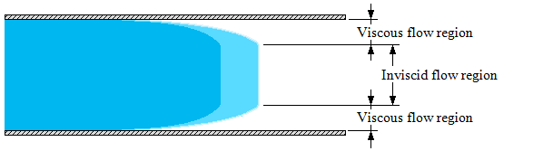
Solver Study: Inviscid and Laminar Models
Inviscid Flow

An inviscid flow is the flow of an ideal fluid that is asumed to have no viscosity. In fluid dynamics there are problems that are easily solved by assuming that the flow is inviscid. It is a flow in which the viscous effects can be neglected.
The flow of fluids with low values of viscosity agree closely with inviscid flow everywhere except close to the fluid boundary where the boundary layers plays a significant role. At high reynolds numbers, flow past slender bodies involve thin boundary layers. Viscous effects are important only inside the boundary layer and the flow outside it is nearly inviscid. If the boundary layer is not separated then the inviscid flow model can be used to predict the pressure distribution with reasonable accuracy.
The inviscid flow model in ansys fluent can be used for simulations where nature of flow in not important to the problem like all the simple heat flow problems. Although air flow on an aircrafts body in with very high reynolds numbers(nearly inviscid) but the assumption of completely ignoring viscosity result in poor results and create problems while analysing high lift devices or analysis at high AOA. For better results the laminar flow model should be used.
Laminar Flow

Laminar flow is a type of fluid flow in which the fluid travels on smooth or in regular paths, in contrast to turbulent flow, in which the fluid undergoes irregular fluctuations and mixing. In laminar flow, sometimes known as streamline floe, the velocity, pressure and other flow properties at each point in the fluid remain constant. Laminar flow over a horizontal surface may be thought of as consisting of thin layers, or laminae, all parallel to each other, The fluid in contact with the surface is stationary, but all the layers slide over each other.
For eg. Laminar flow in a straight pipe may be considered as the relative motion of a set of concentric cylinders of fluid, the outside one fixed at the pipe wall and the others moving at increasing speeds as the centre of the pipe is approached. Smoke rising in a straight path from a cigarette is undergoing laminar flow. After rising a small distance, the smoke usually changes to turbulent flow , as it eddies and swirls from its regular path

An inviscid flow is the flow of an ideal fluid that is asumed to have no viscosity. In fluid dynamics there are problems that are easily solved by assuming that the flow is inviscid. It is a flow in which the viscous effects can be neglected.
The flow of fluids with low values of viscosity agree closely with inviscid flow everywhere except close to the fluid boundary where the boundary layers plays a significant role. At high reynolds numbers, flow past slender bodies involve thin boundary layers. Viscous effects are important only inside the boundary layer and the flow outside it is nearly inviscid. If the boundary layer is not separated then the inviscid flow model can be used to predict the pressure distribution with reasonable accuracy.
The inviscid flow model in ansys fluent can be used for simulations where nature of flow in not important to the problem like all the simple heat flow problems. Although air flow on an aircrafts body in with very high reynolds numbers(nearly inviscid) but the assumption of completely ignoring viscosity result in poor results and create problems while analysing high lift devices or analysis at high AOA. For better results the laminar flow model should be used.
Laminar Flow
Laminar flow is a type of fluid flow in which the fluid travels on smooth or in regular paths, in contrast to turbulent flow, in which the fluid undergoes irregular fluctuations and mixing. In laminar flow, sometimes known as streamline floe, the velocity, pressure and other flow properties at each point in the fluid remain constant. Laminar flow over a horizontal surface may be thought of as consisting of thin layers, or laminae, all parallel to each other, The fluid in contact with the surface is stationary, but all the layers slide over each other.
For eg. Laminar flow in a straight pipe may be considered as the relative motion of a set of concentric cylinders of fluid, the outside one fixed at the pipe wall and the others moving at increasing speeds as the centre of the pipe is approached. Smoke rising in a straight path from a cigarette is undergoing laminar flow. After rising a small distance, the smoke usually changes to turbulent flow , as it eddies and swirls from its regular path
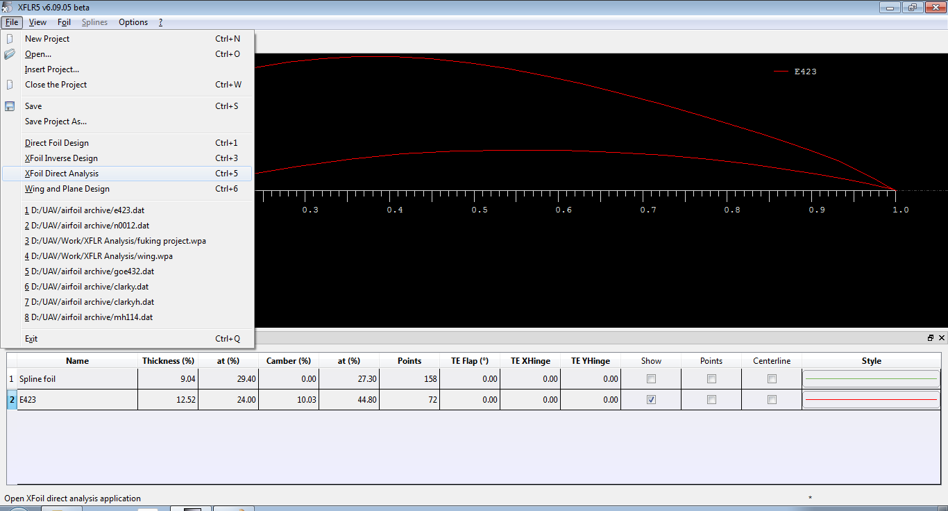
Airfoil Analysis in XFLR
Airfoil Analysis in XFLR
- Design The airfoil in XFLR


- Define The analysis


- Get the final graphs


Making Mould in SolidWorks
Making Mould in SolidWorks
- Open the part file of the object to be moulded

- Make Parting Line.

- Make Parting Surface


- Make axis to define direction vector for ruled surface

- Make bottom Surface of mould and trim the surface with the ruled surface to create the bottom of the mould

- Make the tooling split


- Split the final mould


Mixing of hot and cold water CFD
MIXING OF HOT AND COLD WATER CFD
- CAD :
The geometry is a simple 2 inlet pipe with a mixing junction and an outlet. Cold Water enters from one end and combines with hot water coming from the second end at the junction both inlets are velocity inlets and the outlet is pressure outlet set to zero. (NOT A WALL)
- MESHING :
Learned the importance of slicing up the geometry


Unsliced Geometry


Unsliced Geometry Mesh

Sliced up geometry


Sliced up geometry mesh
- Running the solution :
1) check the mesh
2) Enable the energy equation and k-epsilon models
3) set the boundary conditions for the inlet and the outlet and also specify their temperatures
4)Intialise the solution and run the calclations - Results:
Cold velocity inlet= 0.05m/s hot velocity inlet= 0.05m/sCold water temperature = 300KHot water temperature = 400K


Making Composite Templates
Composite Templates were made in order to calculate their gsm (grams per square meter) so that their strength could be determined which helps in deciding, what kind of composite should be used to make a particular part of a plane. Vacuum bag moulding was used to make the templates.
Materials Used:
- 400 gsm Carbon fiber

- 100 gsm e glass fiber

- 200 gsm e glass fiber

- DIAB divinycell

- Araldite AY 105 epoxy with HY 991 hardener (10:1)
- Felt (breather cloth) : It is used for absorbing the excess epoxy that is pulled up by the vacuum pump.
- Teflon coated glass fiber (Separator): It is used for separating the breather cloth from the epoxy covered CF/GF layers and prevents them from sticking to each other.

- Vacuum bag

- Double sided butyl tape (Tacky tape) : It is used for sealing the vacuum bag.


- Clean the moulding surface and apply 2 coats of mould releasing agent.
- Make the vacuum bag and seal it from all sides but one which will be used to insert the laminates.
- Cut the required pieces of breather and separator.
- Measure the required amount of epoxy and its hardener.
- Begin layup by applying epoxy on the moulding surface. (The amount of epoxy on the first layer must be more than the others so that it can be sucked up by the vacuum).
- Place the required layers one by one covering them with just enough epoxy so as to wet the layers completely.
- Place the separator followed by the breather after all the layers have been layed up
- Place the templates inside the vacuum bag and seal the bag.
- Start the vacuum pump to begin the process.
- Check for any leaks and make sure that a sufficient amount of vacuum is established.


